
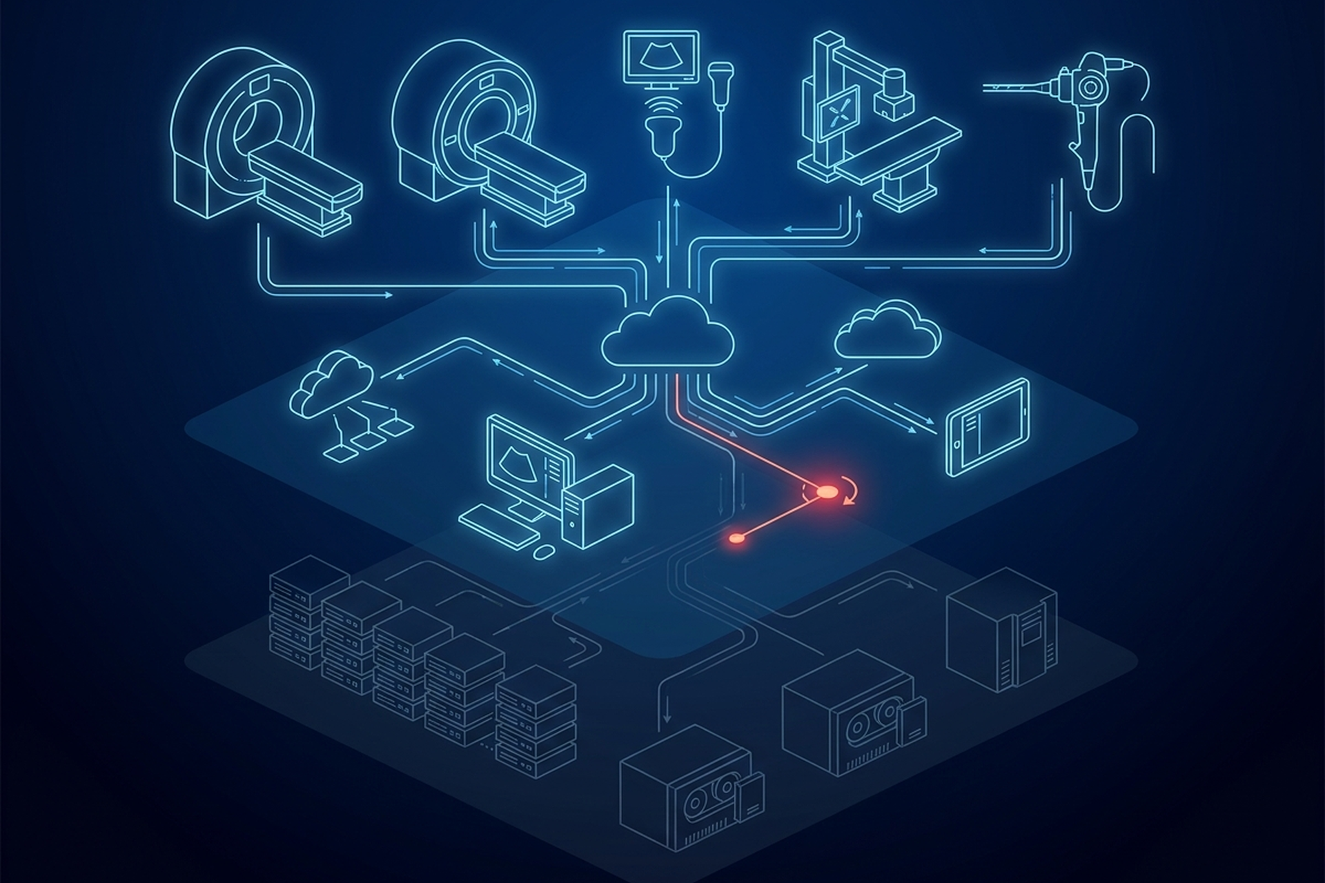
Ask a product team how much storage their imaging platform needs, and the estimate starts with an average: a typical study size, times studies per day, times the years of retention. That number is wrong more often than not, and not by a rounding error. Real medical imaging storage solutions have to size for a distribution, not a mean: a handful of modalities and protocols generate most of the bytes, and retention is set by law rather than preference. Get the distribution wrong and the storage line item either runs out mid-contract or gets built two or three times larger than it needed to be.
What follows is the arithmetic: what drives a single study’s size, why an average across modalities hides more than it reveals, and how a retention window turns a per-study number into a multi-year total. Tiering and compression come last: one changes what a byte costs, the other changes how many bytes there are, and neither replaces the total.
Why the Average Study Size Is the Wrong Number
Averaging treats every study as interchangeable. It isn’t. A two-image chest X-ray and a multi-sequence MRI are both “a study,” but they are nowhere near the same number of bytes. Blending them into one figure hides exactly the information a sizing decision needs.
The skew shows up even inside a single modality. One published account of a hospital’s CT dataflow found that thin-section volumetric reconstructions accounted for close to three-quarters of the CT service’s total storage load. The thick-section images radiologists actually read day to day accounted for roughly a quarter, and both came off the same raw acquisitions. Two datasets, same scanner, same patient, same exam: one of them was the minority of the bytes and the majority of what got read.
That is the shape of the problem at every level. A DICOM object carries its pixel data as a product of four attributes: rows, columns, frames, and samples per pixel, multiplied by the bytes each sample is allocated. Slice count sits one level up, multiplying that per-object figure across however many objects a protocol produces. Change any one of those and the byte count moves by a multiple, not a percentage.
What Actually Drives a Single Study’s Size
Cross-sectional modalities like CT and MRI typically encode one DICOM instance per slice, so a single study is not one file. It is however many slices the protocol called for, each instance carrying its own complete header alongside its share of the pixel data. A routine protocol with a few dozen slices and a fine-cut protocol with several hundred are both “a CT,” and their byte counts are nowhere near the same.
Ultrasound and endoscopy usually go the other direction. A cine loop or a procedure recording lands as a single multi-frame object, one instance holding dozens or hundreds of frames end to end. Its size scales with frame count and duration rather than with a slice tally. A ninety-second cine run and a four-second one are both “an ultrasound clip.”
Bit depth compounds both patterns. The standard allocates pixel data in whole bytes per sample, so an image stored at more than eight bits per sample takes two bytes where an eight-bit image takes one. That doubling lands on every pixel of every frame, before compression ever enters the picture.
None of that is exotic once it is named. The honest sizing question is never “how big is a study.” That question has no answer at the catalog level. It is “how many slices or frames, at what bit depth, for this specific protocol,” asked once per category a partner’s platform actually handles.
The Arithmetic: From Bytes Per Study to Total Archive Size
The same published CT dataflow study measured actual per-study byte counts instead of a vendor’s estimate. Across a sample of abdominal CT volumetric datasets, image count per study ranged from a few hundred to well over a thousand. The resulting data volume ranged from roughly 230 MB to nearly 850 MB uncompressed, for what was nominally the same protocol on the same scanner. A single average drawn from that range would misrepresent almost every individual study it was supposed to describe.
Sizing medical imaging storage solutions correctly means running the multiplication once per category, not once overall: bytes per study, times studies per year, times the years retention requires. Run it for each modality and protocol the platform stores, then sum the categories: a catalog with five modalities is five separate calculations, not one. Skip the breakdown and a storage estimate quietly inherits whichever category dominated the sample used to build it, rarely the category that dominates at real volume.
That product is not the size of the archive on day one, when it holds nothing. It is the cumulative total at the end of the retention window, and it is only correct if the annual study count stays flat for every one of those years. It never does. Volume grows, so the honest version of that term is not one flat studies-per-year figure times the retention years: it is the sum of each year’s actual study count across the window.
Growth Over the Retention Window
Growth is not evenly distributed across modalities any more than size is. One peer-reviewed study tracking a hospital’s archived imaging volume over an eleven-year period found total archived data growing roughly 200 percent. The growth was wildly uneven by modality: archived ultrasound volume grew by more than 400 percent over the period, while archived X-ray volume grew by less than 10 percent. So the studies-per-year term is a curve per category, not one blended rate applied to the whole catalog.
That unevenness is not abstract for a platform serving more than one department, either. The moment a new service line starts sending studies into a shared archive, it brings its own growth curve with it. A storage model built around the original department’s numbers never accounted for that curve, and consolidating imaging across departments tends to force the question sooner or later.
Who Actually Sets the Retention Clock
Retention is the single largest multiplier in the whole calculation, and it is not the platform’s to set. The common assumption that HIPAA fixes a retention period for medical images does not hold up. HHS’s own answer is that state laws generally govern how long medical records are kept, and the period varies by jurisdiction and often by record type. Generally is not always: Medicare’s conditions of participation set a federal floor of at least five years for a hospital’s medical records, and a state or a study type can require longer.
A vendor neutral archive evaluation runs into this directly: retention has to be configurable per jurisdiction and per study type. Whatever period a vendor shipped as a convenient default is not a legal answer. So the retention-years term is not a number a product team gets to pick for convenience: it has to reflect the study types and jurisdictions a partner actually operates in. Building to the shortest plausible figure to keep an estimate small is building to a number the archive will not legally be allowed to use.
Tiering: What “Cold” Actually Costs
None of this means every byte needs to sit on the fastest, most expensive storage for the full length of its retention window. A study read last week and a study read five years ago do not need the same retrieval speed. Separating recent, actively referenced studies from older ones that are rarely retrieved is standard practice once volume justifies it.
Tiering changes what a byte costs, not how many bytes there are, so the total from the arithmetic stays exactly where it was. What gets underpriced is retrieval: a cold tier is optimized for cost per byte at rest, and that optimization has a mirror-image cost on the way back out. Access is slower when an older study does get pulled, whether that is a returning patient, a malpractice request, or a research query years after the fact.
How fast a study has to come back is a requirement to specify up front, the same way how a study performs over a wide area connection is. A tiering policy that never gets tested against an actual cold retrieval is a policy nobody has verified.
Compression Trade-offs: Where Lossy Is Not an Option
Compression is the other lever, and unlike tiering it does change the byte count, within a hard limit. In the same published CT dataflow, image data was typically “compressed in the range 2.5:1 to 3:1 in a lossless manner,” meaning every pixel value reconstructs exactly on decompression. That is a real, meaningful reduction, and it costs nothing in fidelity.
Lossy compression buys more reduction than that, at the cost of changing the pixel values permanently. DICOM’s own standard defines a compressed image whose pixel data differs enough to affect professional interpretation as a new, separate object, not a smaller version of the same one. It also tracks the change for the life of the object: once an image’s Lossy Image Compression attribute has been set to indicate lossy compression, “it shall not be reset.”
That is the practical boundary. Lossy compression has a real place in preview, triage, or referral copies where a fast look matters more than diagnostic-grade fidelity. It has no place on the primary archival copy of a study a signed report depends on. Permanently altered pixel data that cannot be un-flagged is precisely the property an archive copy cannot have.
What This Means for Sizing Medical Imaging Storage Solutions
The arithmetic has three terms: bytes per study, studies per year, and retention years, run once per category and summed. Bytes per study comes from rows, columns, frames, samples per pixel, bit depth, and how many objects the protocol produces, which is why one blended study size describes no modality accurately. Studies per year is a curve, not a constant, so it has to be summed across the window per category rather than multiplied flat. Retention years comes from law, not from what is convenient to build to.
Tiering and compression come after the total, not instead of it. Tiering changes what a byte costs; lossless compression changes the byte count without touching fidelity; lossy compression stays away from the copy of record. Price the retrieval side of a cold tier before committing to it, not after.
None of that sizing work is something a PACS decides on a partner’s behalf. What EBM mAIn PACS® provides is the layer underneath it: native DICOM services (C-STORE, Query/Retrieve, Modality Worklist, and Storage Commitment), the vocabulary every imaging product in the chain has to speak. They do different jobs: C-STORE moves a study into an archive, Query/Retrieve gets it back out, and Storage Commitment is how the archive accepts custody of what it was sent. Modality Worklist sits before any of that: the RIS, or a broker in front of it, exposes the scheduled procedure step through its DICOM Modality Worklist service, and the modality queries it before acquisition.
EPS Pi stores studies with local backup via USB at the point of care, which is a different question from how a long-term archive gets tiered and sized across its full retention window. That is its own layer of the platform, evaluated on the arithmetic above and on whatever care-setting solution it ends up serving, not assumed from a vendor’s brochure.